By Steve Saxton 

Microsoft Excel continues to evolve, offering powerful tools that simplify data manipulation and analysis. Among the latest additions are the TAKE, DROP, and FILTER functions, which provide users with unprecedented flexibility and efficiency in handling data. Here’s a closer look at how these functions work and their potential impact on your workflow. 

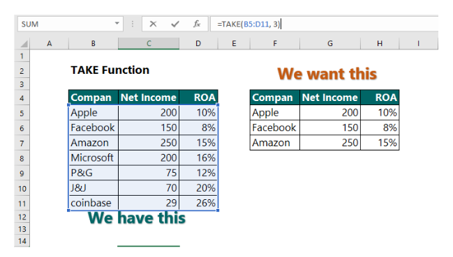
TAKE Function: Extracting Data with Precision 

The TAKE function is designed to extract a specific number of rows or columns from an array, either from the beginning or the end. This function is particularly useful when you need to focus on a subset of your data without altering the original dataset. 

Syntax: 

=TAKE(array, rows, [columns]) 

array: The range of cells from which you want to extract data. 

• rows: The number of rows to take. A positive number extracts from the start, while a negative number extracts from the end.
• columns (optional): The number of columns to take. Similar to rows, a positive number extracts from the start, and a negative number from the end.

Example: To extract the first three rows from a dataset in range A1:C10: 

=TAKE(A1:C10, 3) 

DROP Function: Simplifying Data by Exclusion 

The DROP function complements TAKE by allowing you to remove a specified number of rows or columns from an array. This function is ideal for excluding unwanted data, making your dataset more manageable. 

Syntax: 

=DROP(array, rows, [columns]) 

• array: The range of cells from which you want to drop data.
• rows: The number of rows to drop. A positive number drops from the start, while a negative number drops from the end.
• columns (optional): The number of columns to drop. A positive number drops from the start, and a negative number from the end.

Example: To remove the first two rows from a dataset in range A1:C10: 

=DROP(A1:C10, 2) 

FILTER Function: Dynamic Data Filtering 

The FILTER function is a game-changer for dynamic data analysis. It allows you to create a new array that includes only the rows that meet specified criteria. This function is invaluable for generating reports and insights from large datasets. 

Syntax: 

=FILTER(array, include, [if_empty]) 

• array: The range of cells to filter.
• include: A logical test that determines which rows to include.
• if_empty (optional): The value to return if no rows meet the criteria.

Example: To filter out rows where the value in column B is greater than 100: 

=FILTER(A1:C10, B1:B10 > 100, “No results”) 

Conclusion 

The introduction of the TAKE, DROP, and FILTER functions marks a significant enhancement in Excel’s data manipulation capabilities. These functions empower users to handle data with greater precision and efficiency, making complex tasks simpler and more intuitive. Whether you are a data analyst, a business professional, or a casual user, mastering these functions will undoubtedly elevate your Excel skills.